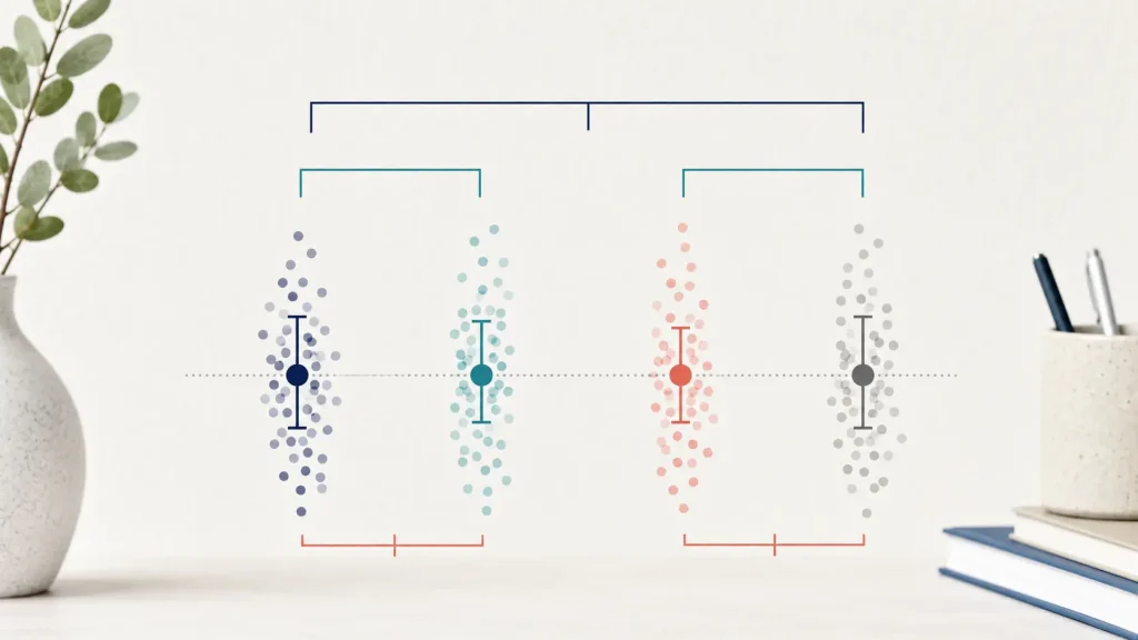
Psychology dissertation planned contrasts translate theory-led predictions into specific comparisons among group means. They help you test the questions that motivated your design instead of relying only on an omnibus ANOVA or examining every possible pair after seeing the results.
A credible contrast analysis begins before the focal results are inspected. You must define the target means, choose interpretable weights, align each contrast with the fitted model, address multiplicity, and report estimates with uncertainty. This guide explains that workflow through psychology-specific examples while separating planned contrasts from post hoc comparisons and ordinary factor coding.
What are psychology dissertation planned contrasts?
A contrast is a linear combination of model-based means. In a simple one-factor experiment with three groups, it can compare one group with another or compare one group with the average of two groups. The coefficients express the comparison. For a conventional difference contrast, the coefficients sum to zero.
Suppose a student compares a wait-list group, a brief intervention, and an extended intervention. A contrast with weights minus 2, 1, and 1 compares the wait-list mean with the average of both intervention means. A second contrast with weights 0, minus 1, and 1 compares the two intervention durations. Multiplying every weight by the same constant changes the numerical scale of the estimate but not its test statistic.
The Leibniz Psychology record on planned contrasts describes their value for linking a priori psychological hypotheses to statistical tests, including hypotheses involving interactions. That alignment is the main reason to use them.
Why an omnibus ANOVA is not the final answer
An omnibus F test evaluates whether the model contains some variation among the relevant means. It does not identify which theory-led pattern produced that variation. A significant result may be driven by a comparison that was not central to the hypothesis. A non-significant omnibus result does not automatically make a prespecified contrast meaningless, although the testing strategy and error control must be stated in advance.
Planned contrasts can focus power on a small number of interpretable questions. They also produce an estimated difference, standard error, confidence interval, and test for each prediction. This is more informative than treating the factor as a single yes-or-no finding.
The site’s psychology dissertation ANOVA guide explains model selection and assumptions. Use it for the underlying design, then use this article to define and interpret the comparisons within that model.
| Analysis | Question answered | Best use |
|---|---|---|
| Omnibus factor test | Do any relevant means differ? | Broad factor-level inference |
| Planned contrast | Does a specified linear combination differ from zero? | Prespecified theoretical prediction |
| Post hoc pairwise comparison | Which pairs differ after broad inspection? | Exploratory follow-up with multiplicity control |
| Trend contrast | Do ordered levels follow a linear or curved pattern? | Meaningfully ordered, suitably spaced conditions |
Define the hypothesis before choosing weights
Begin with a sentence that names the population means. For example: “Participants receiving either active sleep intervention will report lower fatigue than participants receiving sleep information only.” The comparison is active treatments versus control, not three unrelated pairwise tests.
Next, decide whether the two active conditions should contribute equally. Equal weighting may be defensible if the theory treats them as two examples of the same intervention family. It is not defensible merely because the software makes equal weights convenient. Unequal weighting requires a clear substantive reason and changes the estimand.
Record the hypothesis, group order, coefficients, outcome, time point, model, alpha level, and multiplicity strategy in a preregistration or analysis plan. The psychology dissertation preregistration guide can help distinguish confirmatory tests from later exploratory work.
Construct contrast weights correctly
For a difference contrast among cell means, positive coefficients identify one side of the comparison and negative coefficients identify the other. Zero excludes a group from that contrast. Coefficients should normally sum to zero so that the estimate represents a difference rather than an average level.
Balance the two sides of the comparison
If one group is compared with the average of two groups, the absolute weights must balance. Weights 1, minus 0.5, and minus 0.5 compare the first mean with the average of the second and third means. Weights 2, minus 1, and minus 1 express the same test on a scale twice as large.
Do not give a larger coefficient to a group simply because it has more participants. Contrast weights define the scientific comparison, while sample sizes enter the standard error. In an unbalanced design, estimated marginal means can provide model-adjusted comparisons, but their reference grid and weighting still require explanation.
Check the group order
A correct vector attached to the wrong factor order tests the wrong hypothesis. Print the factor levels and contrast matrix before fitting the model. Label every coefficient in a table rather than relying on memory. This simple check is essential when data have been imported with alphabetical ordering or recoded categories.
| Hypothesis for four groups | Example weights | Interpretation |
|---|---|---|
| Control versus all three interventions | -3, 1, 1, 1 | Average intervention mean minus control mean, scaled by three |
| Brief versus extended treatment | 0, 1, -1, 0 | Direct difference between two selected conditions |
| Two individual formats versus two group formats | 1, 1, -1, -1 | Average format difference, scaled by two |
| Linear trend across equally spaced doses | -3, -1, 1, 3 | Monotonic linear component across dose levels |
Always state the group order beside the weights. A coefficient vector without labels cannot be audited reliably.
Understand orthogonal and nonorthogonal contrasts
Two contrasts are orthogonal in a balanced design when the sum of the products of their corresponding weights is zero. Orthogonal contrasts partition independent components of the factor’s model sum of squares. With three group means, at most two linearly independent contrasts are available; with four means, at most three are available.
Orthogonality can be useful, but it is not a scientific goal by itself. Two important hypotheses may overlap and therefore be nonorthogonal. Do not replace a meaningful comparison with an artificial one merely to make the coefficient products sum to zero.
Unequal sample sizes complicate simple textbook statements about orthogonality and sums of squares. Model-based tests should use the actual covariance structure. Describe whether your contrasts refer to raw cell means, equally weighted marginal means, or population-weighted marginal means.
Choose coding that represents the intended question
Contrast coding and planned comparisons are related but not identical. Factor coding determines how model coefficients represent levels of a categorical predictor. A planned contrast may be tested directly as a linear function of fitted means even when the model uses another coding scheme.
The UCLA Statistical Methods guide to contrast coding demonstrates treatment, deviation, Helmert, reverse Helmert, adjacent-difference, polynomial, and user-defined systems. The right choice depends on the comparisons implied by the research question.
- Treatment coding compares each non-reference level with a chosen reference level.
- Deviation coding compares levels with a mean-of-means reference.
- Helmert coding compares a level with a defined average of subsequent or previous levels, depending on the convention.
- Successive-difference coding compares adjacent ordered levels.
- Polynomial coding evaluates trend components across ordered levels.
- Custom coding represents theory-specific comparisons that standard schemes do not provide.
Software conventions differ, especially in the direction and scaling of Helmert or difference coding. Never infer meaning from the label alone. Inspect the matrix and verify the estimate against the intended means.
Use polynomial contrasts only for defensible trends
Polynomial contrasts separate ordered means into linear, quadratic, and higher-order components. They are suitable when factor levels represent a meaningful order and the scores used for the trend represent the spacing among levels.
For equally spaced exposure durations of 0, 10, 20, and 30 minutes, an equally spaced linear contrast can be reasonable. For durations of 0, 5, 20, and 60 minutes, default equally spaced coefficients test a trend across category positions, not a linear trend in minutes. Use scores that match the actual spacing or model duration as a continuous predictor when appropriate.
Do not apply polynomial contrasts to nominal groups such as therapy schools, nationalities, or recruitment sites. Their ordering would be arbitrary and the resulting linear or quadratic component would have no stable interpretation.
The official R documentation for contrast matrices describes built-in treatment, sum, Helmert, and polynomial functions. It also shows that contrast matrices have one fewer contrast column than factor levels when used for factor coding.
Plan psychology dissertation planned contrasts and multiplicity
Calling a test “planned” does not automatically remove the risk created by many tests. Define the family of claims and justify how its error rate will be controlled. A small number of genuinely prespecified, distinct contrasts may be analysed under a focused confirmatory strategy. A long list that covers most possible patterns is functionally exploratory.
State whether each contrast is a separate primary hypothesis or whether several contrasts jointly support one conclusion. If any significant contrast can establish the main claim, the familywise error rate may need control. If all prespecified components must be significant, the decision rule differs. Secondary outcomes, time points, subgroups, and alternative models can expand the family even when each contains only one contrast.
Holm adjustment is a general familywise procedure when several hypotheses form one confirmatory family. Other methods may be justified by the dependence structure or a specialised comparison set. False discovery rate control may be suitable for a clearly exploratory family but does not provide the same claim-level protection as familywise control.
Use the psychology dissertation multiple-comparisons guide to define families and select an adjustment. Avoid presenting unadjusted exploratory contrasts as if they were the only tests conducted.
Fit contrasts within the correct model
A contrast inherits the assumptions and estimand of the fitted model. For a between-participants experiment, independence follows from the design, not from a diagnostic test. Residual behaviour, variance structure, influential observations, clustering, missingness, and outcome scale still matter.
In ANCOVA, compare adjusted means at a stated covariate reference or averaging rule. In repeated-measures and multilevel models, account for dependence rather than running separate one-way analyses at every time point. For generalised linear models, explain whether contrasts are reported on the link scale or transformed response scale.
Estimated marginal means are particularly useful for interactions, covariate-adjusted models, and unbalanced data. The emmeans documentation explains how model predictions are averaged over a reference grid and how contrasts can be computed for many linear, generalised linear, mixed, ordinal, and other models. The averaging weights and transformation scale remain substantive choices.
Test planned interaction contrasts
A theory may predict that a group contrast changes across another factor. This is a contrast of contrasts. For example, an intervention-versus-control difference may be expected to be larger under high stress than low stress. The target is the difference between those two intervention effects, not two separate claims that one simple effect is significant and the other is not.
Write the cell-level hypothesis before entering coefficients. For a two-by-three design, label all six cells and form the interaction contrast from the relevant simple contrasts. Check that the final weights match the desired signs and that excluded cells have zero weight only when the hypothesis truly excludes them.
Do not infer an interaction because one simple contrast has p below .05 and another has p above .05. Directly test their difference and report its estimate and confidence interval.
Worked psychology dissertation example
Consider an experiment on memory retrieval with three study conditions: restudy, retrieval practice, and retrieval practice plus feedback. The first prediction is that the two retrieval conditions will outperform restudy. The second is that adding feedback will improve performance beyond retrieval practice alone.
Using the order restudy, retrieval, retrieval plus feedback, the first contrast can use weights minus 2, 1, 1. The second can use 0, minus 1, 1. Their cross-product is zero, so they are orthogonal in the balanced three-group design. Together they represent the two degrees of freedom for the group factor.
The student fits the planned model, checks the group order, calculates estimated differences, and reports intervals. Suppose the first contrast estimate on the chosen scale is 12.0 percentage points with a 95% confidence interval from 7.0 to 17.0. The scaled estimate must be translated carefully: if weights minus 2, 1, and 1 were used directly, divide by the relevant scaling factor before describing an average treatment-versus-control difference.
Suppose the second estimate is 3.0 points with a confidence interval from minus 1.0 to 7.0. The data support a retrieval-versus-restudy advantage but remain compatible with small negative and positive feedback effects. The result does not prove that feedback has no value. An equivalence test with justified bounds would be needed for a bounded absence claim.
| Reporting element | What to provide | Why it matters |
|---|---|---|
| Hypothesis | Named means and expected direction | Connects the test to theory |
| Weights | Labelled vector in exact factor order | Makes the comparison auditable |
| Estimate | Difference in interpretable units | Shows magnitude and direction |
| Uncertainty | Standard error and confidence interval | Shows precision |
| Inference | Test statistic, degrees of freedom, p-value, adjustment | Documents the decision rule |
| Model context | Covariates, random effects, scale, averaging rule | Defines the estimand |
Report planned contrasts clearly
In the method section, explain when the contrasts were specified, list the coefficients and group order, identify the model, and state the multiplicity strategy. Describe any robust standard errors, degrees-of-freedom method, transformation, or estimated-marginal-means reference grid.
In the results section, report the contrast estimate in meaningful units, its uncertainty, test statistic, degrees of freedom where applicable, p-value, and effect size when useful. If coefficients were scaled for calculation, present an estimate readers can interpret. Include a compact table for several contrasts.
In the discussion, interpret the contrast rather than restating significance. A positive intervention-family contrast supports the predicted average difference under the specified model. It does not establish that every intervention group differs from control unless that was tested. A non-significant contrast indicates uncertainty, not equivalence or proof of no difference.
Check your software output
Retain syntax and software versions. Print factor levels, contrast matrices, estimated marginal means, and the coefficient vector passed to the testing function. Recalculate simple contrasts from displayed means when feasible. This detects reversed signs, unintended reference groups, and scaling mistakes.
For SPSS, distinguish built-in contrast options from custom linear hypotheses and verify the order used by the procedure. For R, distinguish factor coding in the model matrix from post-fit contrasts of estimated means. A model coefficient may answer the planned question only if the coding and interactions make that interpretation valid.
When sharing code, remove private participant data and absolute file paths. Preserve a synthetic example or a documented contrast table so another researcher can reproduce the hypothesis without accessing confidential records.
Common mistakes to avoid
- Choosing contrasts after inspecting group means while calling them confirmatory.
- Attaching correct weights to the wrong factor-level order.
- Using weights that do not represent the verbal hypothesis.
- Interpreting a scaled coefficient as an unscaled mean difference.
- Assuming all planned tests can be left unadjusted regardless of number or role.
- Using polynomial trends for nominal or unequally spaced levels without justification.
- Testing simple effects separately instead of directly testing an interaction contrast.
- Ignoring dependence, clustering, missing data, or unequal variances in the fitted model.
- Reporting only p-values without estimates, intervals, or contrast definitions.
- Claiming no difference from a non-significant contrast.
Frequently asked questions
Must planned contrast weights sum to zero?
For a conventional difference among means, yes. Zero-sum weights remove the common level and define a comparison. Some regression parameterisations use different coding conventions, so interpret the exact model matrix rather than applying a rule mechanically.
Do planned contrasts require a significant omnibus ANOVA?
Not necessarily. A prespecified contrast can directly test the hypothesis it was designed to represent. State the planned inferential strategy in advance and do not use the omnibus result selectively to decide which contrasts to report.
How many independent contrasts can I test?
A factor with k levels has k minus one linearly independent contrast dimensions. You can calculate more comparisons, but they will not all be independent and multiplicity still requires attention.
Are orthogonal contrasts always better?
No. Orthogonality can partition information cleanly, especially in balanced designs, but scientific relevance comes first. Important hypotheses may overlap and therefore be nonorthogonal.
What is the difference between contrast coding and a planned contrast?
Contrast coding parameterises categorical predictors in a model. A planned contrast is a specific hypothesis about means or model predictions. It can often be tested after fitting the model, regardless of the original coding, if the linear function is correctly specified.
Can planned contrasts be used with mixed models?
Yes. Contrasts can be applied to model-based predictions or estimated marginal means from a suitable mixed model. Report the random-effects structure, degrees-of-freedom method, averaging rule, and scale.
Should I adjust p-values for planned contrasts?
It depends on the number, dependence, and decision role of the tests. Define the hypothesis family and error criterion before analysis. A label such as “planned” is not by itself a multiplicity solution.
Conclusion
Psychology dissertation planned contrasts provide a disciplined route from theoretical predictions to interpretable group comparisons. Define the means, weights, scale, model, and error-control strategy before inspecting results. Then verify the matrix, report estimates with intervals, and keep exploratory comparisons clearly labelled.
If you seek dissertation support, choose ethical tutoring that helps you understand, check, and reproduce your own analysis. Keep responsibility for the hypotheses, code, interpretation, and final writing, protect participant information, and follow your institution’s rules on permitted assistance.